Basic Views:
Parasternal long axis view (PLAX)
The parasternal long axis view is commonly the first view obtained in an echo examination and is useful for assessing contractility visually, assess mitral and aortic valves, calculating ejection fraction in M-mode, detecting regional wall motion abnormalities, measuring LV outflow tract diameter for cardiac output studies and identifying pericardial effusion.
Parasternal short axis view (PSAX)
-
The parasternal short axis view at the level of the aortic valve is used to look for vegetations, and other abnormalities of aortic valve structure.
-
The parasternal short axis view at the level of the mitral valve is used to measure mitral valve area.
-
The parasternal short axis view at the papillary muscle level is useful for assessing the LV end diastolic area (an index of volume status), visual gestalt assessment of contractility, detecting regional wall motion abnormalities, detecting right ventricular enlargement and assessing interventricular septum motion abnormalities in acute cor pulmonale.

Short axis view at the level of the papillary muscles
Short axis view at the level of the aortic valve
Apical 4 chamber view (A4C)

The apical 4 chambered view is used to detect and quantify mitral and tricuspid regurgitant and stenotic lesions using color flow imaging and Doppler. It is also used to detect right ventricular enlargement, visually assess RV and LV contractility, calculate ejection fraction using the 2D method, assess mitral and tricuspid inflow patterns and measure pulmonary vein inflow for diastolic function.
Apical 5 chamber view (A5C)
Transducer position and marker dot direction are same as the A4C view. The A5C view is obtained from the A4C by slight anterior angulation of the transducer towards the chest wall. The 5th chamber added is the LVOT.
The apical 5 chambered view is used to measure LV ouflow tract velocities to measure cardiac output. It is also useful to detect and quantify aortic regurgitation and stenosis using color flow imaging and Doppler.

Apical 2 chamber view (A2C)
Marker dot direction: points towards left side of the neck (45-60 degrees anti-clockwise from A4C view)

Apical long axis or 3 chamber view (A3C)
The transducer is placed at the same position as for a A4C view and then turned clockwise by 60°. You can also obtain the three-chamber view by rotating the transducer even further in counterclockwise direction from the two-chamber view (approximately a further 60°).
It is similar to a parasternal long axis view seen from the apex and characterized by the presence of the mitral and aortic valves in the same plane. The apical 3 chambered view is used to measure LV outflow tract velocities when the A5C is suboptimal.

Sub costal view

The inferior vena cava (IVC), descending aorta, interatrial septum and pericardial effusions are best seen in this view. This view is also particularly useful when obesity, emphysema or chest wall deformity prevents satisfactory transthoracic views from being obtained.
It is used to measure IVC variability to assess volume status, diagnose small pericardial effusions, and measure RV free wall thickness to diagnose chronic cor pulmonale.
Remember to change the depth, as the heart is usually 22 cm from the probe surface in the subxiphoid view but closer in the parasternal and apical view.
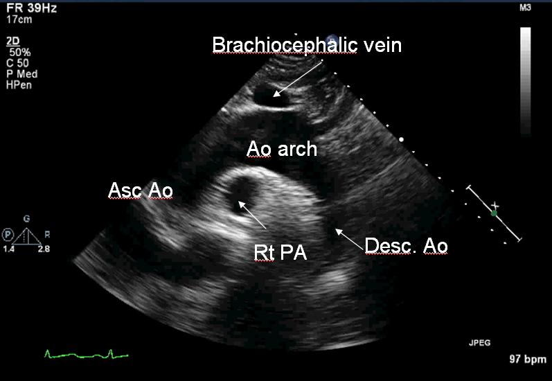
Suprasternal Long axis view:
Have the patient lie completely flat without anything under the head. Ask them to lift their chin upward and look to the left. Then place the transducer in the suprasternal notch with the probe pointed at the left shoulder at about 2 o'clock.
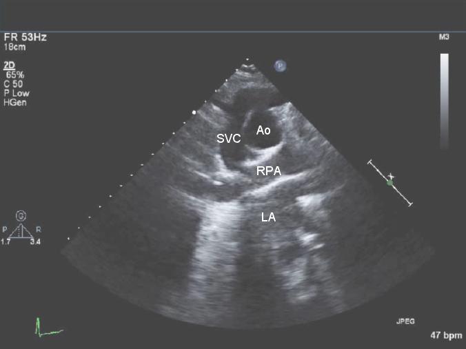
Suprasternal short axis view:
Turn the probe clockwise to the 5 o'clock position, roughly perpendicular to the long axis view.
Segments or walls of Heart

Volume status:
IVC diameter and variability
After obtaining a 2-D image of the IVC entering the right atrium and verifying that the IVC visualization is not lost during movements of respiration, place an M-mode line through the IVC 1 cm caudal from its junction with the hepatic vein, and obtain an M-mode tracing. This placement ensures that we do not measure the intrathoracic IVC during any part of the respiratory cycle.
If the patient is spontaneously breathing, ask him to take a short quick inspiratory effort ("a sniff") during the M-mode recording. If the patient is mechanically ventilated, record the M-mode through 3 or 4 respiratory cycles.
Low CVP is increasingly likely as IVC diameter (IVCD) gets smaller than 1 cm and abnormally high CVP increasingly likely as IVC diameter increases above 2cm. The IVC size is an indicator of volume status and not volume responsiveness – these two are not the same.
IVC collapsibility index
In a spontaneously breathing, healthy subject, cyclic variations in pleural pressure, which are transmitted to the right atrium, produce cyclic variations in venous return, which is increased by inspiration, leading to an inspiratory reduction of about 50% in IVC diameter.
The IVC collapsibility index is expressed as the difference between the value of the maximum diameter and the minimum diameter, divided by the maximum of the two values. It should be noted that the denominator here is the maximum diameter. This index is used only for spontaneously breathing non ventilated patients. This is an index of volume status (hypovolemia, hypervolemia) and right atrial pressure.
IVC distensibility Index:
In a patient requiring ventilatory support, the inspiratory phase induces an increase in pleural pressure, which is transmitted to the right atrium, thus reducing venous return. The result is an inversion of the cyclic changes in IVC diameter, leading to increases in the inspiratory phase and decreases in the expiratory phase.
This variation is quantified by measuring the difference between the maximum and minimum diameters on the M-mode tracing and dividing it by the mean of the two. This is referred to as ΔIVC. It should be noted that the denominator here is the mean diameter. In mechanically ventilated patients, a 12% or more variation identified patients likely to respond to volume.
Some others use another index called the distensibility index. This differs from ΔIVC in that the denominator is the minimum diameter. The cutoff for this index is 18%.
Left Ventricular end diastolic area (LVEDA)
First, obtain a 2-D parasternal short axis view at the level of the papillary muscles. Freeze it and scroll back and forth to identify a frame showing the left ventricle in end diastole. You can use the ECG to time this. Using a caliper, trace along the endocardium to measure the area of the left ventricle at end diastole. You do not have to trace around the papillary muscles and they can be included inside the circle.
An LVEDA of less than 10cm2 indicates significant hypovolemia. An LVEDA of more than 20cm2 suggests a volume overload.
Another sign that suggests severe hypovolemia is the "kissing papillar muscle sign" where opposing papillary muscles come in contact with each other at end systole.
One thing to remember is that severe concentric hypertrophy can reduce LVEDA even without any hypovolemia.
Left ventricular outflow tract (LVOT) Velocity Time Integral (VTI) variation with respiration
In the apical 5-chamber view, place a PWD sample volume in the middle of the LVOT just adjacent to the aortic valve. The sample cursor should not overlie the valve. Obtain a PWD tracing. Make sure there is no valve opening artifact in front of the systolic flow waveform. That means that the cursor is placed over the aortic valve and needs to be moved into the LVOT by a few millimeters.

Once you have obtained the waveform over 3 or 4 respiratory cycles, freeze the image. Reducing the horizontal sweep speed enables capture of a larger number of LVOT ejections. Scroll back and forth till you can identify the largest (usually at end inspiration, if mechanically ventilated) and the smallest waveforms over a single respiratory cycle. Go to ‘calculations'…'aortic continuity equation'….'LVOT VTI' and trace the edge of the waveforms using the trackball.

The machine will calculate the VTIs for these two waveforms. The VTI variation is then calculated as the difference between the maximum and the minimum VTI divided by the mean of the two values.

Measuring the maximum and minimum Vmax at the LVOT
A VTI variation of more than 12% predicts fluid responsiveness (defined as an increase in cardiac output by at least 15% in response to a standard fluid bolus).
Left ventricular outflow tract (LVOT) Velocity Time Integral (VTI) increase with Passive Leg Raise (PLR)
The LVOT VTI is measured with a PWD in the A5C view as described above with the patient in semi-recumbent position (head up 45°). 2 assistants then lift both lower limbs of the patient to a 45° angle. A repeat LVOT VTI is measured after 1 minute.
Passive leg elevation (PLR to 45°) induced increase in VTI by > 12% predicts an increase in stroke volume by > 15% after saline infusion (500ml over 15minutes).
Pulsed Wave Doppler (PW)
PW allows us to measure blood velocities at a single point, or within a small window of space. It requires the ultrasound probe to send out a pulsed signal to a certain depth (chosen by the operator) and then stay quiet and just listen for the reflected frequency shift from that particular depth. The computer then calculates the velocity of flow at the chosen point. Because the machine has a waiting time to listen for a return, there is limit to how fast it can accurately measure the velocity of blood flow.

This is an example of PW at the left ventricular outflow tract (LVOT) in the apical long axis. You are seeing the machine plot velocities (y axis shown in cm/s) over time (x axis). Each velocity is plotted as one white point. Many white points (from many doppler shift frequencies) make up the nice flow profile shown above. The more intense the density of white points, the stonger the signal returning to the probe at the frequency/velocity.
The baseline is shown as an orange line going across. Points below the line represent velocities going away from the transducer. Points above the orange line show velocities going toward transducer. So we can deduce from above that there is a pulsatile flow going away from the transducer in systole (right after the QRS on the EKG tracing in green).
LV systolic function/ Ejection Fraction:
M-mode LV dimensional method:
First obtain a parasternal long axis view and place an M-mode cursor is placed through the septal and posterior LV walls just beyond the tip of the mitral leaflets.
In the resultant M-mode image take measurements of the RV internal dimension, interventricular septum thickness, LV internal dimension and LV posterior wall thickness at end-diastole (timed on ECG or point of largest LV internal dimension) and at end-systole (ECG timed or point of smallest LV internal dimension).
In the resultant M-mode image take measurements of the RV internal dimension, interventricular septum thickness, LV internal dimension and LV posterior wall thickness at end-diastole (timed on ECG or point of largest LV internal dimension) and at end-systole (ECG timed or point of smallest LV internal dimension).

With this information, most machines will be able to generate two numbers, the fractional shortening and the ejection fraction.
While the M-mode method of calculation of EF is easy to learn and perform, it has some drawbacks. The M-mode assessment provides information about contractility along a single line. In a patient with coronary artery disease and regional wall motion abnormalities, the severity of the dysfunction may be underestimated if only a normal region is interrogated or overestimated if the M-mode beam transits through the wall motion abnormality exclusively.
2-D method of Simpson
In this method, acquire A4C or A2C views, making sure that the endocardial borders are visualized well. Freeze the image and scroll backward and forward to identify a frame at end diastole. This can be timed using the appearance of the ventricle – identifying a frame where the ventricle appears to have the largest volume; or with the ECG trace, where the peak of the R wave corresponds to end-diastole.
Open the "calculations" menu and select "LV volumes" and "A4C diastolic" or "A2C diastolic", whichever is appropriate. Place the cursor on the endocardial border where the anterior mitral leaflet meets the interventricular septum and trace the entire endocardial border of the left ventricle. You do not have to trace around the papillary muscles. Once this is done, the LV volume in diastole will be calculated.

Drawbacks: It is sometimes difficult to place the probe at the exact apex to get a full view of the LV cavity. This leads to foreshortening of the LV cavity and underestimation of LV volumes.
Doppler assessment of cardiac output
First measure the LVOT diameter on a Parasternal Long Axis view. This is done by zooming into the LVOT on the PLAX view using the zoom tool and freezing the image. The images are scrolled backward and forward to capture a frame in which the aortic valve leaflets are wide open. The LVOT diameter is measured adjacent to the points of attachment of the leaflets. The machine will then calculate the cross sectional area (CSA) of the LVOT.
Next, obtain an apical 5-chamber view of the heart. As mentioned earlier, the A5C view is obtained from the A4C by slight anterior angulation of the transducer towards the chest wall. The 5th chamber added is the LVOT. Place the Pulsed Wave Doppler cursor in the LVOT as close to the aortic valve as possible without including it in the sample volume. Acquire the PWD trace.

Then choose LVOT VTI from the "calculation" menu and manually trace the PWD waveform. Some machines may be able to do this automatically. The machine will calculate the area under the curve and represent it as a Velocity Time Integral (VTI) in cms. Repeat the VTI measurement thrice to reduce sampling bias.
- The stroke volume at the LVOT is then obtained by multipying the LVOT VTI with the LVOT cross sectional area.
- LVOT VTI x LVOT cross sectional area = Stroke volume
- Stroke volume X Heart rate = Cardiac output
Drawbacks:
-
Sometimes an adequate A5C view may not be obtainable. In such a case, an apical 3-chamber view can be tried.
-
The LVOT may not be aligned with the direction of the PWD, leading to underestimation of velocities. In this situation, an apical 3-chamber view may sometimes offer better alignment.
-
When the parasternal long axis view is not obtainable, a LVOT diameter of 2cms for males and 1.75cms for females can be assumed.
Right heart assessment:
Detection of RA and RV enlargement
Parasternal short axis view
Typically this view shows the round LV with the thin, crescenteric RV cavity anterior and to the right of it hugging the round LV contour. The RV cavity cross section is smaller than the LV cavity cross section.
Typically this view shows the round LV with the thin, crescenteric RV cavity anterior and to the right of it hugging the round LV contour. The RV cavity cross section is smaller than the LV cavity cross section.
When the RV dilates, 2 things are noticed. First, the RV cross section becomes as large as, or larger than the LV cross section. Secondly, the RV cavity becomes more rounded with the IVS moving into the LV cavity during part (early diastole) or whole of the cardiac cycle. This causes the typical round cross section of the left ventricle to become "D-shaped".

Also, septal flattening is seen in right heart failure. Septum becomes flat in systole or both systole/ diastole in increased right sided pressure overload and flattening is seen in diastole in volume overload.
Apical 4 chamber view
Normally, the right ventricular cavity is usually 2/3rd of left ventricular cavity in this view. The RV can be said to be significantly enlarged if the RV cavity appears to be as large as or larger than the LV cavity on this view. In addition, the RV loses its usual triangular shape and becomes more oval. In severe RV enlargement, the RV apex may extend beyond the LV apex.
RV systolic function- Tricuspid annular plane systolic excursion (TAPSE)
In an Apical 4 chambered view, an M-mode cursor line is paced through the lateral tricuspid annulus and an M-mode tracing is obtained and frozen. A sinusoidal line representing the motion of the annulus is noted. Measure the amount of longitudinal displacement of the annulus at peak-systole.

Normal value for TAPSE: above 1.6 cm
RV systolic function- Tricuspid annular displacement (TAD)
In an Apical 4 chambered view, a M-mode cursor line is paced through the lateral tricuspid annulus and a M-mode tracing is obtained and frozen. A sinusoidal line representing the motion of the annulus is noted. Using calipers, the distance from the peak to the trough of this wave is measured. This distance is the TAD.
In an Apical 4 chambered view, a M-mode cursor line is paced through the lateral tricuspid annulus and a M-mode tracing is obtained and frozen. A sinusoidal line representing the motion of the annulus is noted. Using calipers, the distance from the peak to the trough of this wave is measured. This distance is the TAD.
Normal TAD is >1.75 cm.
References: www.criticalecho.com
PEARLS:
-
Pericardial versus pleural effusion: Pericardial effusion is usually located circumferentially. If the echo free space is seen only anteriorly, it is more likely an epicardial pad of fat or a pleural effusion. Posteriorly a pericardial effusion is anterior to the descending thoracic aorta whereas a pleural effusion is posterior to it. If pericardial and pleural effusions co-exist, then a linear echo (the pericardium) separates them.
-
Pericardial Tamponade: RV collapse in early diastole and RA collapse in late diastole and early systole is highly sensitive. Left atrial collapse is highly specific for cardiac tamponade.
-